
How to Set up a Dynamic Water Recycle Calculation
From Enersight version 2.14 onwards, expanded functionality regarding drilling step conditions and Job Material results being available mid-calculation have enabled dynamic re-calculation of water costs and schedule timing to be evaluated within a single pass. This removes the need to calculate the model, extract results, transform and reload key scheduling limitations then recalculate, iterating until second and third order downstream effects are resolved, significantly reducing overall calculation time and the need for manual intervention.
This topic outlines a few examples demonstrating how to:
- Charge your system inflow water requirements
- Limit your scheduling based upon available water
Water available, but at a cost
The first case models an asset where extra water may be purchased to top up the required amounts to retain the desired frac schedule.
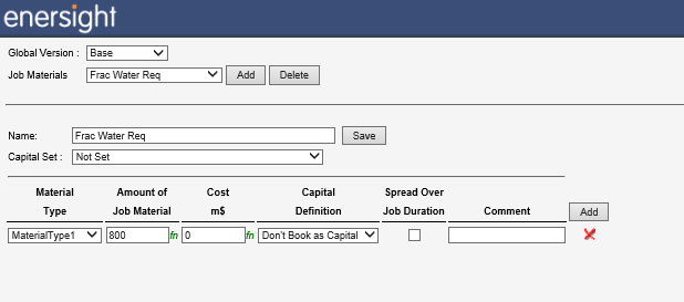
To initiate the tracking of the required water to complete the well, a Job Material of ‘Frac Water Req’ has been defined by accessing the below screen via Enterprise > Manage Job Materials. In this case it is 800 units of water, representative of 800 mbbl of overall water. This could alternatively be defined as a function utilizing key details of the wells such as lateral length, number of stages etc. to determine the requirement.
Click image to expand or minimize.
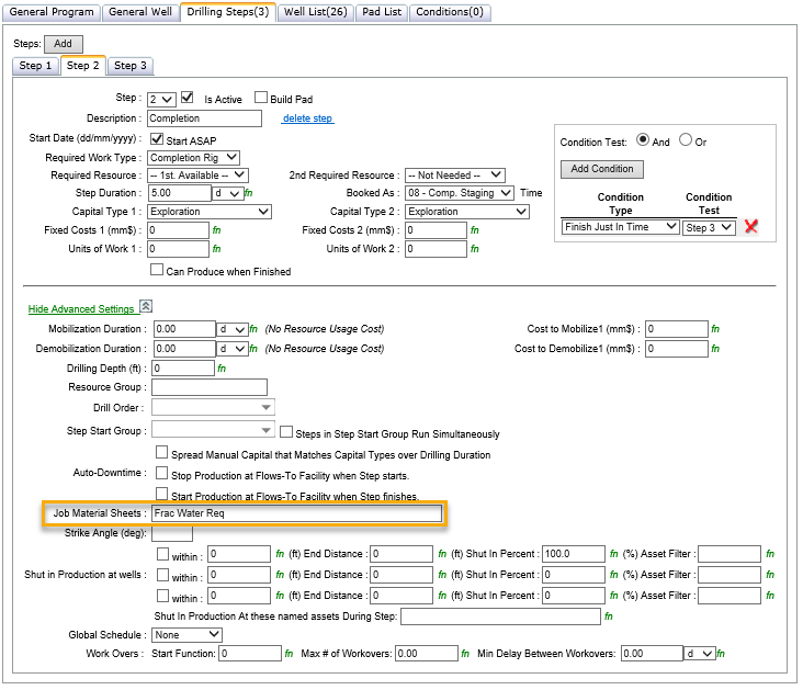
This Job Material is then assigned as part of the Drilling Step, in this case specifically being placed on the Completion Step.
Click image to expand or minimize.
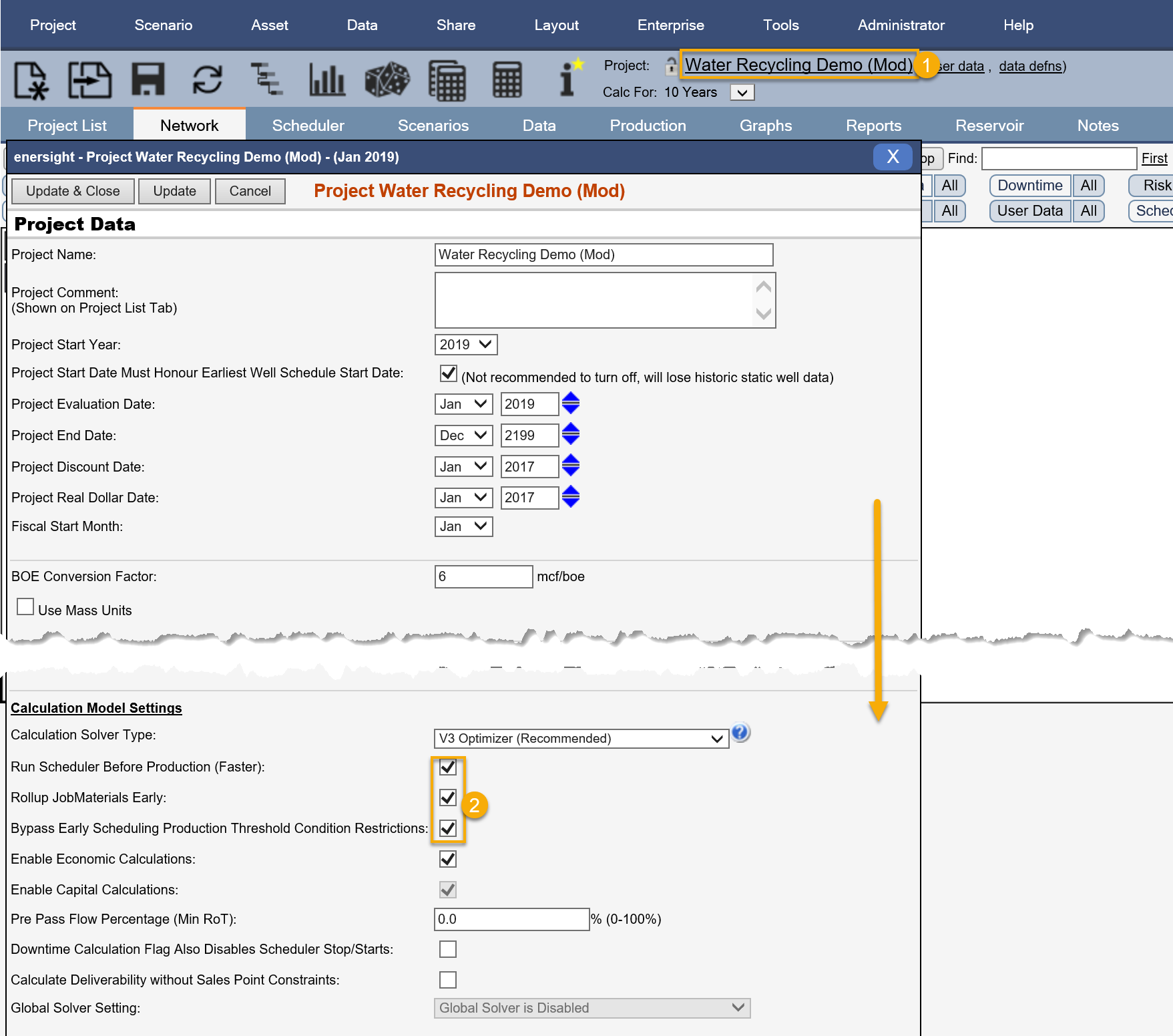
In order to have the calculation see the Job Material results, some project level settings now need to be adjusted to ensure that these items flow through the calculation process at the right time. Note that whilst the 'Bypass Early Scheduling Production Threshold Conditions Restrictions' is not required for the first example case, it is necessary for the second example and doesn't hurt to be ticked regardless.
Click image to expand or minimize.
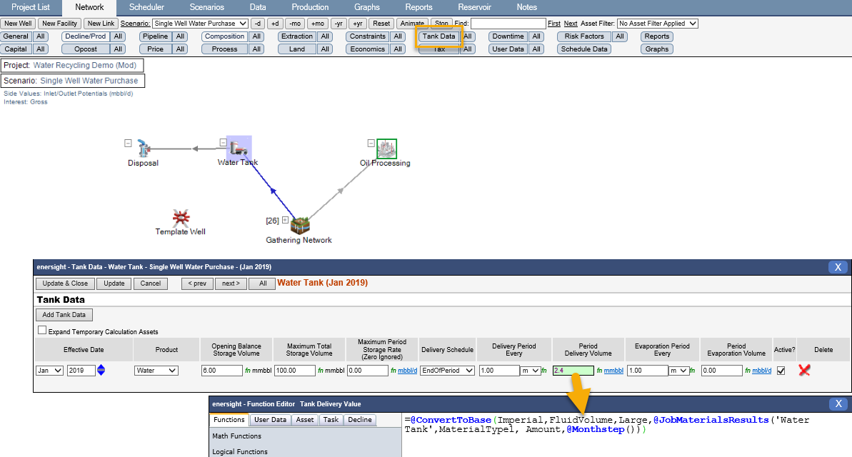
Now within the network, the available water produced is sent to the Water Tank asset which has a tank constraint defined. In your model you may have other water uses, sources (i.e., rain forecast) and / or losses from processing which you need to include – these elements should be able to remain as is, with just the tank storage asset requiring updating as per below. Key inputs for this tank include the starting balance, a maximum storage as well as a delivery schedule which looks at the amount of Job Materials generated by the Frac Water Required.
Click image to expand or minimize.
In this specific example the model is being run monthly and thus the delivery period is specified monthly – in the case of a daily approach then this can be adjusted along with the function to use @JobMaterialsResultsDaily().
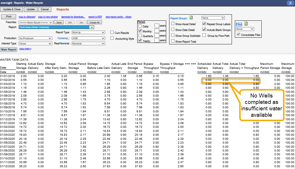
Once the model has been run you will be able to analyze the scheduled delivery against actual throughput via the Tank Data (Water Volumes) report. In the below case it identifies that for March 2019 that insufficient actual total deliveries and throughput were available to meet the scheduled requirement.
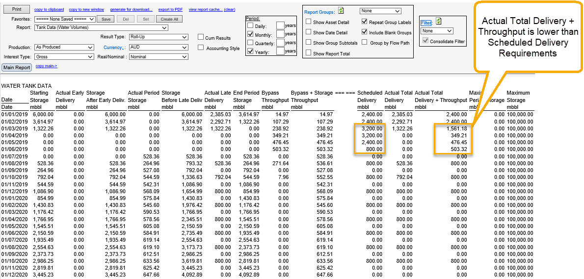
Click image to expand or minimize.
The cost of this shortfall can be generated at the disposal node that the water flows to using a fixed per month operating cost that compares the Job Material Requirements with the available delivery of water from the tank and then applies a rate, in this case $0.50 per barrel on any purchases required to top up.
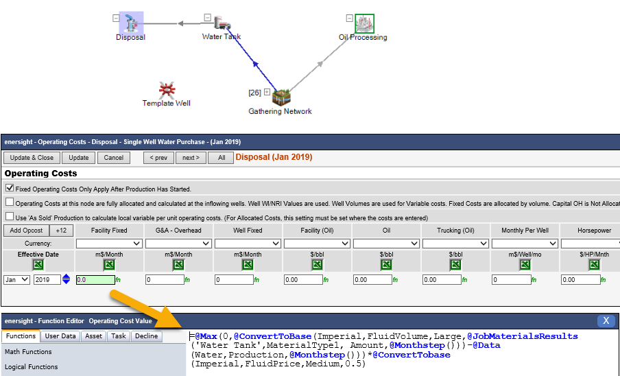
Click image to expand or minimize.
A summary report can then be created to simplify future analysis of the required top up water relative to overall requirements and the associated incremental costs via creating a customized report.
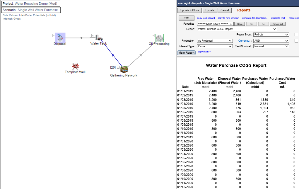
Click image to expand or minimize.
Limited water available, affecting the scheduled timing of wells
The second case models an asset where no extra water is available and the frac schedule needs to be adjusted to ensure it complies with this requirement.
This case also uses the same ‘Frac Water Req’ however it also introduces a couple of Production Threshold conditions on the schedule so as to ensure that it only proceeds with activities when there is sufficient water available within the tank of ‘Water Tank’ and that the oil produced can be utilized at ‘Oil Processing’.
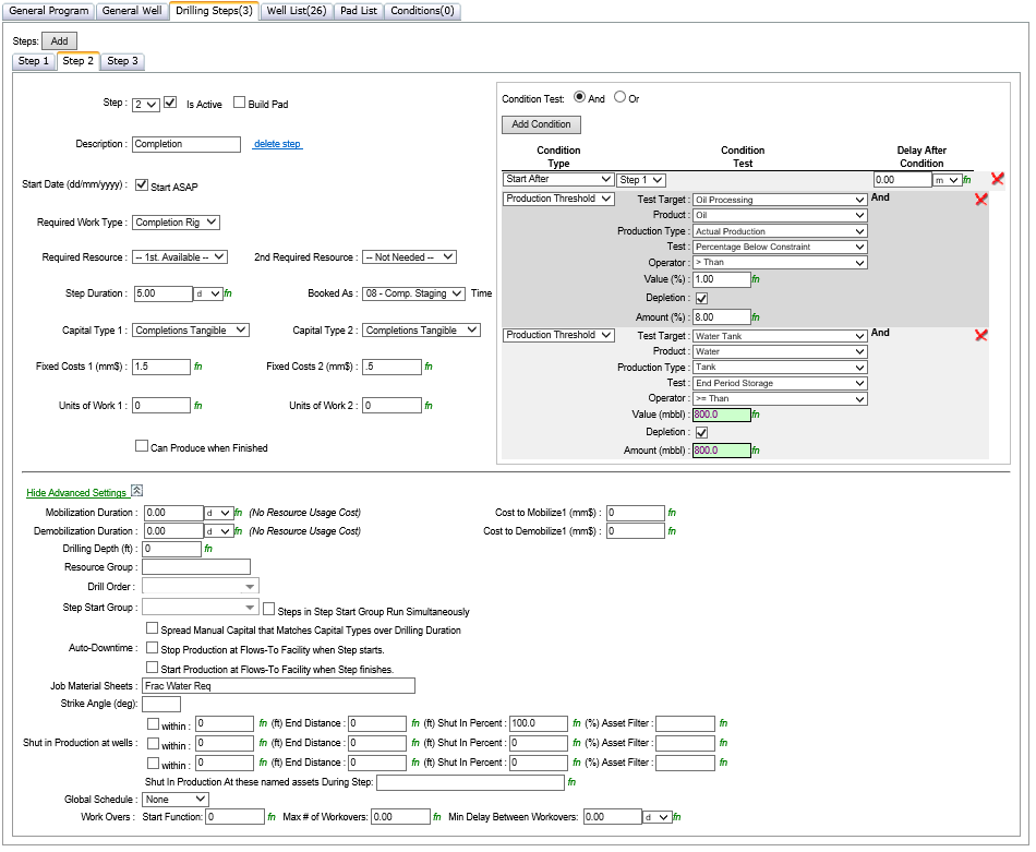
Click image to expand or minimize.
In this case the amount of Water being check for and depleted is a function referring to the amount of Job Materials that would be required IF the step went ahead via “=@ConvertToBase(Imperial,FluidVolume,Large,@TaskConditionJobMaterials(0))”. The depletion amount here is matching the ‘Water Tank’ Delivery volume using the same function as the previous example. The settings for the Oil Processing will depend on the relationship between the peak production of the wells relative to the constraint and could be tuned over time to give the appropriate fit.
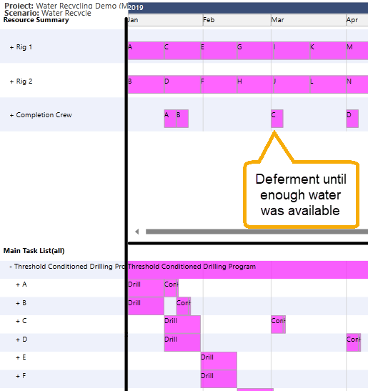
Similarly to the first example, the results of the Tank Data (Water Volumes) may be reviewed in conjunction with the Gantt Chart to ensure that wells were only completed when sufficient water was available.
Click image to expand or minimize.
Click image to expand or minimize.
The above setup works also for step groups, where sufficient materials must be available for the entire step group prior to proceeding on the activity.